7964
Lecture 11

In this discussion, we'll focus on regression analysis.

I. Regression

Regression analysis -- when one is just thinking about two variables -- offers us a way to "predict" or "explain" one variable (the dependent variable) with another variable (the independent variable. So, for instance, to use an example we've used before, one could predict undergraduate student grades with class attendance. Undergraduate grades would be the Y variable (the dependent variable, or the "left hand side" variable), and class attendance would be the X variable (the independent variable, or the "right hand side" variable).

In its simplest form, with only two variables -- one dependent (or response) variable Y and one explanatory or independent variable X -- regression analysis essentially plots a line. The formula for any line is:

Y = a + bX

X and Y are variables--they can change value from case to case in your data set. That is, the X for observation 1 (X₁) is not necessarily the same as the X for observation 2 (X₂).

a and b, on the other hand, are constants. They are the same no matter what the value of X and Y.

"a" is the intercept--it is the value of Y when X crosses the Y axis.

"b" is the slope--it is the change in Y associated with a one-unit change in X.

How does this relate to correlation? Well, regression is very much based on correlation. Recall that the Pearson's correlation was a measure of the strength of the linear relationship between two variables. "Ordinary Least Squares" regrssion analysis is a method that just calculates out a slope and an intercept for a line that is plotted to fit the datapoints in the scatter plot.

II. Minimizing squared "errors" to fit the Line

How does OLS (Ordinary Least Squares Regression) fit a line to data? (Note--this is just background information; you don't actually need to know this to do any of the calculations, or to figure out the slope or intercept).

OLS minimizes squared errors. What does this mean? What is an "error"?

For each observation X or case, the error is the difference between the observed Y in your dataset and the predicted Y that falls on the line.

Let's think about an example. Say you have a data set, such as one we examined in lecture 10:



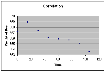
So, for example, the equation for the line that fits the data displayed in the scatterplot above is:

Y (dye weight) = 368.35 + -.039 (X: time in minutes).

(We'll explain below how we calculated out the a and b).

368.35 is the intercept; it is the value of Y when X=0. Notice that this works out algebraically, because if X=0, then -.039*X drops out of the equation, leaving us with Y = 368.35.

-.039 is the slope; the negative sign indicates that it is downward sloping, (or that an increase in X is associated with a decrease in Y). The slope seems quite small in magnitude, but in part that's just because of the range of the Y variables. The slope tells us that for each one unit change in X (that is, for each minute) Y is expected to drop -.039. For the second data point in our set of data, what is the observed Y? Click here for the answer.

But what is the predicted Y for the second data point? You can calculate it out by plugging in X and Y into the line above. Click here for the answer.

But there is some error; the actual observation doesn't fall exactly on the line. "Error" in the world of OLS regression doesn't mean mistake -- it just means that not all the points fall on the line (in fact, in plenty of datasets, none of the points actually fall exactly on the plotted line), and that there's some "error" in prediction.

Recall that the "residual" or "error" or (by common notation) "e" is the observed Y - predicted Y. Calculate out the residual --and click here for the answer. Note that the positive residual indicates that the observed Y is larger than the predicted Y--in other words, that the datapoint would be above the plotted line.

Note that "e", just like X and Y, can change from observation to observation-- in some ways "e" is just a variable, albeit one that is manufactured by the line itself. a and b, however, are constants--they remain the same across the entire data set, because there is one constant line, with one slope and one intercept.

OLS picks the line that would minimize the sum of the squared errors (imagine if you squared each residual, and then added up all the squared residuals across all observations.

III. Extensions: Multiple Regression Analysis

One topic that we won't discuss here (there are other classes you are welcome to sit in on) is multiple regression. In multiple regression, you can "control for" other variables, while testing the effect of one variable on another.

IV. OLS assumptions

OLS relies on a number of assumptions (whether you are using bivariate or multivariate regression):

• OLS assumes that you are modelling a linear relationship. If you have non-linear relationships, you need to transform (just as you logged x and / or y in correlations, you can log x and/or y in regression--see lecture 10).
  
  
• OLS assumes that you've included all relevant variables. After all, the entire point of OLS is to measure the effect of a variable (and draw conclusions about that variable's effect in a population) while controlling for other varibles. If you leave those other variables out, the estimate that you're getting for your effect of a particular variable will be biased--that is, even if you collect an infinite number of samples, and average out the "b" or estimated slope/effect of variable X, that average b will not be = the effect in the population.
  
  Bivariate regression--that is, regression with only one independent variable--almost always violates this assumption.
  
• OLS assumes that you've only included relevant variables. If you include irrelvant variables in a multivariate model, the estimated effects will be unbiased--but you'll be using up available information (because you're estimating the effects of multiple variables), and your standard errors will increase (the effects will bounce around more from sample to sample, with more variance). Therefore your degrees of freedom will go down--and (all other things equal) your effects will become less significant, and it will be less likely that you can reject the null hypothesis.
  
  
• OLS assumes no "autocorrelation"--that is, it assumes that the error terms, from case to case, aren't correlated with each other in some pattern.
  
  
• OLS assumes no "heteroskedasticity"--that is, it assumes that the error terms have constant variance. Put more simply, it assumes that you're explaining just as well in one subset of your data as in others.
  
  Heteroskedasticity is very common in pooled data--for instance, it's just more difficult to explain legislative behavior in some states than in others. Legislative behavior is more predictable in some states than in others. And so, in legislative research, heteroskedasticity is quite common. In sociology, it's more difficult to predict the behavior of the relatively young and the relatively old--again, a heteroskedasticity problem.
  
  Heteroskedasticity can be corrected by weighting your data (another entire semester could be spent addressing this), but it needs to addressed. If heteroskedasticity is not addressed, the estimated effects will be unbiased, but the parameter esimates (the estimated effects may be more or less significant than they should be).
  
  
• OLS assumes that all variables are measured correctly. If you've measured an independent variable with error, than the estimated effects will be biased; if you've measured the dependent variable with error, the results will look less statistically significant than they really are (because the standard errors will be inflated).

That all said, OLS is pretty robust even in the face of mild to moderate violations of these assumptions.

V. Calculating the Slope & Intercept

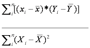
The formula for the slope for the bivariate regression analysis is as follows:



You can calculate out the intercept as follows:

a = (mean of Y) - (b)(mean of X)

So, for the example above, can you use excel to calculate out a slope and intercept? Click here for an excel table that outlines the answer.

VI. Significance Testing for Slopes

How can we do significance testing for slopes?

Given that, generally, we can think of the slope as a sample slope, we can then think about significance testing. We need to find out the standard error associated with our slope. This is the same exact reasoning that we went through when we talked about the mean--we talked about taking an infinite number of samples from our population, calculating a mean from each one--and then the standard deviation of the mean for that hypothetical sample of an infinite number of means is the "standard error".

To review, what does it mean when the standard error is large? Click here for the answer.

What is the formula for the standard error of the slope? First, let's give the formula for the variance of b, and then we can take the square root to get the standard error:



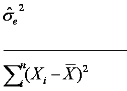
A few points:

• The numerator is just the variance of the error terms--the sigma (lower case) is the notation for "variance", the caret above the sigma represents "predicted" (so we're talking about the standard deviation of the predicted sigma, and the "e" stands for residuals. So, the entire numerator just represents the variance of the residuals, corrected for the degrees of freedom.
  
  
• But how can we calculate out the variance of the residuals? Well, the numerator of the standard error is very similar the variance of the residuals, corrected for the degrees of freedom. That is, the numerator for the variance of the slope can be calculated as:
  
  
  
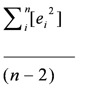
  In other words,
  
  • For each observation, calculate out predicted Y, and calculate out the residual
  • For each observation, square the residuals
  • Then sum up all the squared residuals
  • And divide by n-2 (why n-2? Recall earlier discuss -- you've used up two pieces of information, because you need two points to define a line).
  
  
• Note that the farther the points are from the line, the bigger the variance of the residuals--and therefore, the larger the standard error. The larger the standard error, the more difficult it is to reject the null hypothesis. In other words, as the data points get farther from the line--if there is a "poor fit" of the line to the data--then the standard error is larger, and we expect our slope to bounce around a good deal from sample to sample--and thus are "less confident" when we make inferences about the population.
  
  
• Notice that the denominator is a measure of how spread the X's are around the mean--data that are very well spread out will ahve a larger denominator, and thus a smaller standard error. In other words, the more spread out the X's are around the mean of X, the more stable the slope is--the less we expect it to bounce around from sample to (hypothetical) sample, and the more confident we are in making generalizations about the effect of X on Y (that is, the slope) in the population.

Once we have the stanard error of b, we can calculate

t = b / std error

And use a t-table, just as we've always done.

VII. R-squares

The "R-square" is used to represent the amount of variance in Y explained by X.

In order to caluculate out a R², you go through the following steps:

• For each observation, calcualte out the (Predicted Y - Mean Y)
• For each observation, square that difference between the predicted - mean
• Then, add up all the squared differeces--this is the "Explained some of squares" or "regression sum of squares" (RSS).
• Then, for each observation, calculate out the (Observed Y - Mean Y).
• Then square each of those differences, and sum across all observations. This is the TSS, or total sum of squares.
• The R² is the RSS / TSS.
• Or, it's the square of the Pearson's correlation that you can calculate from your data set.

Note that R² are very useful in terms of measuring the strength of linear relationships, or telling you how much of the variance in Y is "explained" by X.

But, note the limitations of using R²:

• First, correlation is not causation--you need good theory to make predictions. And "b" is actually the appropriate measure of how much "x" affects "y".
• Sometimes people like the R², because like all correlations, it is scaled from -1 to 1. But those are artificial boundaries--a .75 R-square is not always preferable to a .10 r-square.
• The R² is biased in small samples--that is to say, even if you were to gather an infinite number of (small) samples, the average R² would not = the population R².

VIII. Questions

For the data on how weight of dye changes over time, calculate out the variance of b, the t, and the R-square Would you (at a 95% confidence level) reject the null hypothesis that X does not have an effect on Y?