7964
Lecture 10

In this discussion, we'll focus on correlation.

Correlation can be thought of as "strength of relationship" -- that is, if two things are very correlated, they are strongly associated with each other, strongly related to each other. You can generally predict one with a high degree of accuracy if you know the other. So, for instance, class attendance among undergraduates and grades are often highly correlaetd.

However, keep in mind that correlation is merely association--not causation.

Correlation is measured with a "correlation coefficent", which ranges from -1 to 1.

• A correlation of 1 means that two variables are perfectly, positively related-- when one goes up, the other goes up (and when one goes down, the other goes down). "Perfectly" related means that if you know how one variable has changed, you can perfectly predict how the other variable has changed.
• A correlation of -1 means that two variables are perfectly, negatively related; when one goes up, the other goes down (and vice versa). "Pefectly" related means that if you know how one variable has changed, you can perfectly predict how the other variable has changed.
• A correlation of 0 means that there is no relationship between two variables whatsoever. It is virtually impossible for a correlation to be zero--two variables always have some relationship, even if it is very small in magnitude, and entirely random.

Scatterplots--where data are plotted based on two variables, X and Y-- are useful ways to graphically illustrate how correlated two variables are. Click here for examples of positive and of negative correlation.

I. Example #1

Consider the following example, taken from Lucy (2006) (originally taken from Grim (2002)) of data on the average molecular weight of the dye methyl violet and UV irradiation time from an accelerated aging experiment.

Time (minutes	Weight (Da)
0.0	367.20
15.3	368.97
30.6	367.42
45.3	366.19
60.2	365.91
75.5	365.68
90.6	365.12
105.7	363.59

A scatterplot showing the correlation between these two variables would look something like:



The formula for the correlation coefficient is:



The numerator in this formula looks like the variance formula that we've seen for a single variable--but represents the covariance, which is essentially a measure of how much two variables vary together.

The correlation is essentially a standardized version of the covariance--it is the covariance adjusted for the standard deviation of x and y.

What is "r" in example #1? We can calculate out the mean of time as 52.9; we can calculate out the mean of weight as 366.26. Given that,

Time (min)	X - mean X	(X - mean X)2	Weight	(Y - mean Y)	(Y - mean Y)2	(X-mean X)* (Y-mean Y)
0.0	-52.90	2798.41	367.20	.94	.883	-49.72
15.3	-37.61	1414.51	368.97	2.71	7.344	-101.92
30.6	-22.33	498.63	367.42	1.16	1.345	-25.90
45.3	-7.61	57.91	366.19	-.07	.005	.53
60.2	7.33	53.73	365.91	-.35	.122	-2.57
75.5	22.61	511.21	365.68	-.58	.336	-13.11
90.6	37.67	1419.03	365.12	-1.14	1.300	-42.94
105.7	52.84	2792.06	363.59	-2.67	7.129	-141.08

The numerator for "r" is -376.72.
The denominator for "r" is the square root of (18.465 * 9545.49), or 419.83.

The "r" correlation, therefore, is -.8973.

It is negative because as time increases, weight decreases.

II. Significance Testing for Correlations

We can use t-tests to test for significance of a sample correlation.

We calculate

        t =          r X √ df

                   _________________

                      √ (1 - r2)

We've actually used up two pieces of information--we've estimated two means / standard deviations. (You can also think of this in terms of needing or "using up" two data points to plot a line.) So now our "degrees of freedom" are n-2.

So, in this case, the t statistic would = [( -.8973 ) * ( √ 6 )] / ( √ ( 1-.8973² ) = -4.78.

With 6 degrees of freedom, we see that 95% of the t distribution area is within plus / minus 2.447. So, our value of -4.78 is beyond -2.447, so we can say that the linear correlation coefficient is significant at 95% confidence. Indeed, our t tells us that our correlation coefficient is significant even at the 99% level, because the "critical value" of the t at 99% is 3.707--that is, 99% of the area under the t-curve falls between -3.707 and 3.707. Another way to think about this: there's less than a .001 chance that we would get that high of a t if our null hypothesis "no correlation" was true in the population--if these two variables weren't at truly associated with each other in the population.

There are three major limitations of Pearson's correlations:

• First, correlation is not causation--only theory can really give you the information you need to hypothesize causal relationships.
• Second, Pearson's correlations assume that each of the two variables have normally distributed probabilities.
• Third, Pearson's correlations do not capture non-linear relationships.

III. Correlation Coefficents for Non-Linear Data

One complicating issue is that correlation coefficients "r" (these are called Pearson's Correlation Coefficients") only measure linear relationships. Therefore, if you have two variables that are related, but in a non-linear fashion, you may get a deceptively low r, and (in error) fail to reject the null hypothesis. In other words, you may have a relationship, but the Pearson's r fails to give evidence of that relationship.

In order to account for non-linear relationships, you have two options:

• The first is to transform your data. Suppose you have a relationship that looks something like this:
  
  
  
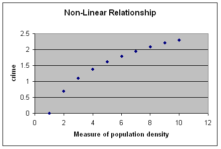
  In this hypothetical example, crime (the y axis) is associated with population density (the x axis)--but not in an entirely linear fashion. While crime increases as population density increases, it actually increases at a decreasing rate.
  
  In order to capture this non-linear relationship accurately, you can transform the variable in the x axis. You need to find a function that mimics the relationship that you have between your x and your y variables. If you can find such a relationship--a relationship between X and function of X that mimics the relationship that you have--you can "convert" you X variable.
  
  This will be more clear if it's applied to an example.
  
  A relationship that "mimics" the (hypothetical) relationship between population density and crime is: the natural log. Indeed, if you plot out X on the X axis, and the "natural log of X" on the Y axis, you'd get the exact same relationship! (It just happens to be *exactly* the same in this example--but you're generally trying to come up with a relationship that has the same basic pattern as the relationship you see or expect to see in your data, even imperfectly).
  
  
  
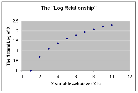
  The log relationship is very, very often used to account for relationships that have one--often very gradual--curve to the relationship. That is, if X is systematically changing as Y changes--but at a (slightly) increasing or decreasing rate--all you need to do is create a new variable, the "log of X", and substitute it in for X.
  
  So, if you had a relationship that looked a bit like the relationship between crime and population denisty, above, all you'd do is
  
  
  • Compute a "new x variable" = log X (in excel, = ln(x)). In the above example, you'd create a new variable which would be the log of population density.
  • Substitute your new x variable in the formula for X.
  • Calculate out the correlation coefficient, and do the appropriate significant testing.
  
  What if you had a relationship that looked a bit like this:
  
  
  
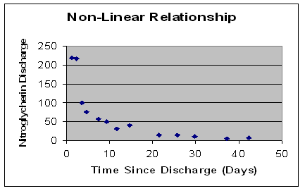
  (in this case, as time since discharge increases, the peak height of nitroglycerin decreases at a decreasing rate-- before, as population density increased, crime increased at a decreasing rate .)
  
  If your relationship looks something like this, you could follow a very similar process as before, but instead transform the variable on the y-axis.
  
  
  • Compute a "new Y variable" = log Y (in excel, = ln(y)). In this case, you'd create a new Y variable which = log of nitroglycerin peak.
  • Substitute your new Y variable in the formula for Y.
  • Calculate out the correlation coefficient, and do the appropriate significant testing.
  
  
• The second option is to use a Spearman Rank Correlation Coefficient.
  
  The Spearman's is an excellent choice for ordinal level data. And, the Spearman coefficient doesn't make any assumptions about how the variables are distributed, and relies less on the assumption of linearity. The Spearman coefficient assumes only that there's a monotonic increase or decrease--so, in other words, as X increases, Y increases (albeit at an increasing or decreasing rate). Most software packages offer the Spearman's as an option.
  
  

  ---

  IV. Partial Correlation

  It is also sometimes useful to calculate out partial correlations-- which are correlations between two variables X and Y that account for relationships to a third variable Z. Partial correlations give us an opportunity to "control for" a third variable, so you can see how two variables are correlated while "partialling out" the effects of a third.
  
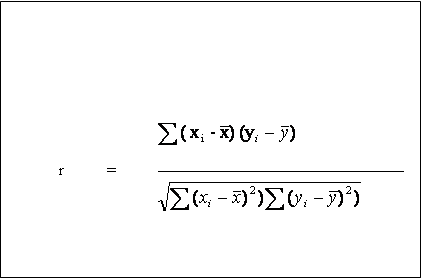
  The general formula for a partial correlation is:
  
  

  r_{ij | k} = numerator / denominator,
  where the numerator:

  r_ij - r_ik*r_jk

  and the denominator:

  √ (1 - r²_ik)*√ (1 - r²_jk)
  
  Where r²_ik, for example, is the correlation between variables i and k.

  
  

  Let's look at an example. Ohtani et al. (2004) measured the D/L ratios for aspartic acid, glutamic acid and alanine in the acid-insoluble, collagen rich fraction from the femur in 21 cadavers of known age at death. The data from aspartic and gluatmic acids is reproduced below:
  
  

  Age	Aspartic	Glutamic
  16	.0608	.0088
  30	.0674	.0092
  47	.0758	.0100
  47	.0820	.0098
  49	.0788	.0092
  53	.0848	.0100
  55	.0832	.0106
  57	.0824	.0098
  58	.0828	.0098
  59	.0832	.0106
  61	.0826	.0108
  62	.0838	.0104
  63	.0874	.0110
  67	.0864	.0106
  67	.0870	.0102
  70	.0860	.0112
  70	.0910	.0112
  72	.0912	.0118
  74	.0932	.0114
  77	.0916	.0110
  79	.0956	.0116

  
  
  Can you fill in the correlation table?
  
  It is:
  
  

  	Age	Aspartic	Glutamic
  Age1.00	.97	.88
  Aspartic----	1.00	.86
  Glutamic----	----	1.00

  
  
  In their paper, Ohtani et al conclude that the D/L ratio of aspartic acid is the most highly correlated of all the amino acids with age. Given that D/L glutamic acid is also highly correlated with age--and given that glutamic acid is also highly correlated with aspartic acide--is this correct?
  
  What partial correlations is the question asking you to calculate?
  
  Which is the largest partial correlation?
  
  

  Click here for the answer.
  
  What is the answer?
  
  Click

  V. Example #2

  Let's look at an example that can be done all three ways: the nitroglycerin example.
  
  

  A. Pearson Correlation

  Time Since Discharge	Nitroglycerin Peak Height
  1.21	218.34
  2.42	216.16
  3.62	100.00
  4.69	75.55
  7.49	56.52
  9.42	50.62
  11.60	31.00
  14.69	41.44
  21.50	15.53
  25.70	14.63
  29.86	10.41
  37.20	5.16
  42.42	7.26

  
  
  What is the correlation based on Pearson's?
  
  Calculate out, and then click here to see the excel spreadsheet with the answer and calculations.
  
  

  B. Pearson Correlation with Transformation to Fit Non-Linear Relationship

  But, we happen to expect--and we happen to know--that the data follow the pattern displayed in the graph above--that the nitroglycerin does decrease with time, but not in a purely linear fashion: it decreases at a decreasing rate.
  
  So, we can transform our "y" variable, nitroglycerin--and create a new y variable, the log of y. (In exel, just calculate out =ln(y).)
  
  We can then recalculate the Pearson's r.
  
  Calculate out, and then click here to see the excel spreadsheet with the answer and calculations. The correlation has increased substantially--indicating that there's an even stronger association between the two variables than we originally thought.
  
  

  B. Spearman Rank Correlation

  Alternatively, we can do a Spearman correlation.
  
  Click here for the appropriation calculations.

  ---

  VI. Question

  Click here for data on a sample of books, including two variables: X=page length, and Y=price of book in dollars.
  
  

  • Create a scatterplot showing the relationship between the two variables. Does it look like there is a relationship?
  • Calculate a Pearson's coefficient.
  • Given the nature of the relationship, replace the X with the log of X, as above, and recalculate the Pearson's. Does the new coefficient indicate that there is a stronger association, once non-linearity is taken into account?
  • Calculate a Spearman's coefficient.
  • Are there any outliers? What would likely happen to your coefficients were you to remove these outliers from the data? Why should you not necessarily make that choice to remove the outlier?